Control voltage, or CV, is one of the things that makes modular synthesizers so appealing to many users. The automating of parameters within the synthesizer and the freedom to patch them in any way you'd like adds to the flexibility of this already free-form instrument. If you want to add some more complexity to your modulation, there are a few methods you can try.
Primarily we'll be looking at control voltage processing in the amplitude domain but will touch on some time-domain manipulation techniques as well. But what does amplitude domain processing look like? And, more importantly, what does it sound like, you may ask?
Amplitude Processing 101: Attenuation and Voltage Amplitude
Amplitude refers to the level of a control voltage—which, in more musical terms, reflects how much change a CV imparts on its destination. This is measured in voltage, commonly expressed as a number followed by V. For example, the standard power connections of a Eurorack modular synthesizer are +12V, -12V, +5V, and ground, sometimes written as gnd, which serves as a 0V reference point for the other voltages. Voltage can exist in both positive and negative forms, which will look at in more depth a little later on.
CV amplitude processing comes in a myriad of forms, each of which alter the behavior and modulation characteristics in distinct ways. A CV signal may be reduced in amplitude, offset to cover a different range of voltages, or combined by addition, subtraction, or multiplication to create a new signal based on the relationship between the sources. Processing the amplitude of a CV source opens up new modulation possibilities, letting you customize the strength or depth of modulation either by hand using knobs or sliders or automated with a secondary (or tertiary) CV signal—allowing for greater nuance and detail in the control of your sounds.
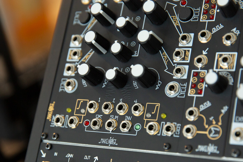
The most basic form of CV processing is attenuation. Attenuation reduces the amplitude of a signal, much like a volume control. Many modules feature built-in input attenuators in addition to parameter control knobs. While sometimes you want broad, sweeping changes to a parameter, sometimes a more subtle approach is necessary. That's where the attenuator comes into play. One good example of this is adding vibrato to an oscillator. You don't typically want the pitch to bounce around a full 10-octave range that could happen with a full-scale +/-5V LFO. Attenuating that signal down to a smaller range provides a more traditional vibrato behavior, a narrow sweep of pitch variation. Attenuation constrains modulation and lets you fine-tune it to your needs.
Attenuverters, Offset, and Inverted Amplitude
Many modules offer a specialized form of an attenuator for some parameters, often referred to as attenuverters (or polarizers). Attenuverters have the ability to both attenuate and invert a signal, depending on the position of the knob. Inversion flips a signal over on itself, changing positive changes in amplitude to negative ones (and vice versa).
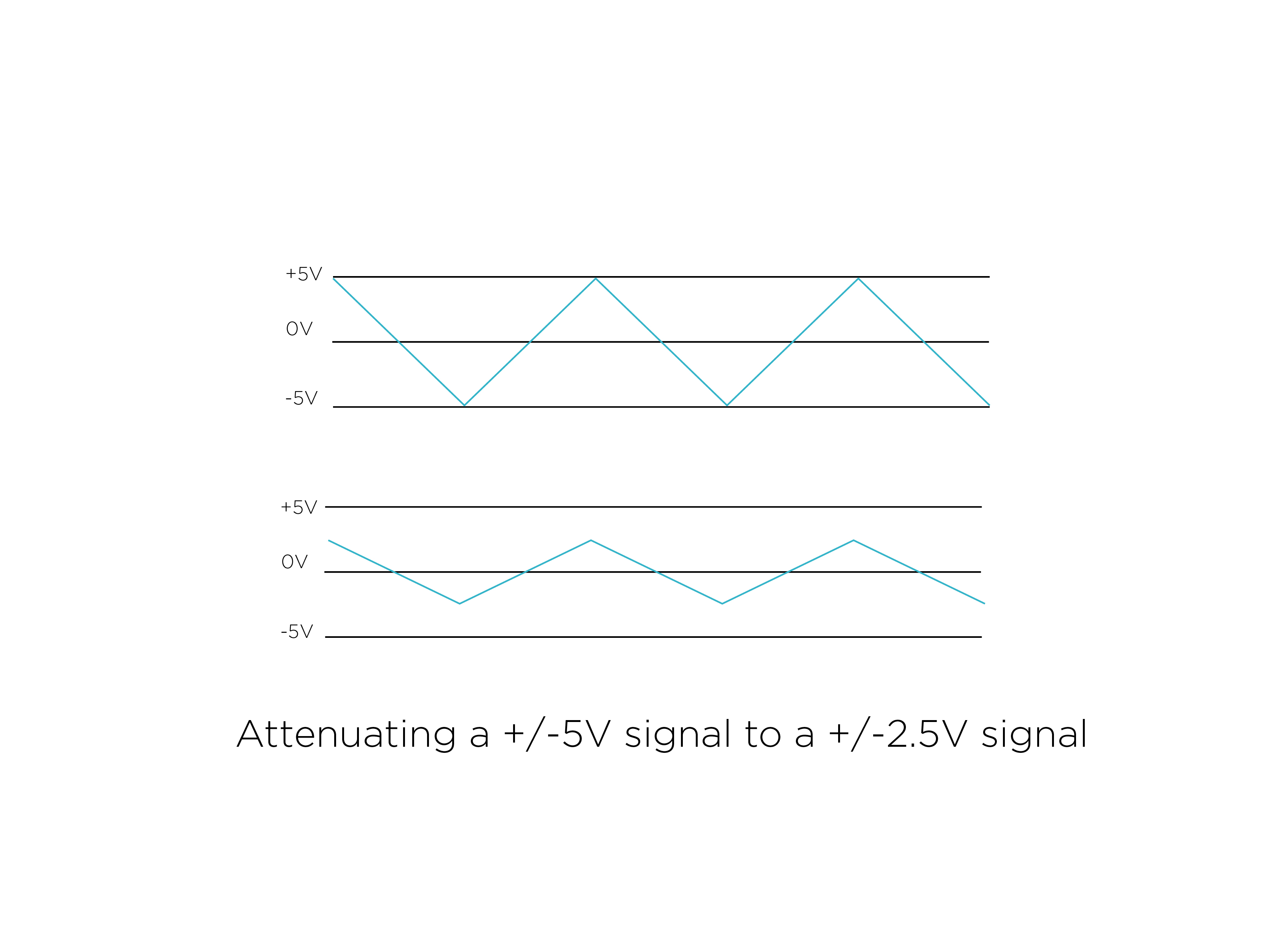
Some of you may be familiar with keyboard synthesizers that feature a reversed envelope for filter modulation, which decreases the filter's cutoff frequency instead of increasing it. If you invert a bipolar signal, the phase flips 180 degrees. For example, the inversion of a falling sawtooth waveform is, as you may have guessed, a rising sawtooth waveform. Instead of ramping down over time and then falling back to the lowest point, the inverted falling sawtooth wave starts at the low point and then travels upward.
In the center of an attenuverter, the signal is effectively off. Turning the attenuverter to the right increases the amplitude of the signal positively while turning to the left increases the signal negatively. "Increases negatively" may sound strange at first, but remember, voltages exist in both the realm of positive and negative. If you have a modulation source patched into an attenuverter and then the 1V/oct input on an oscillator, positive signals make it go up in pitch; negative signals cause it to go down in pitch. Note, not all modules respond to negative voltage changes, including some digital oscillators, most VCAs, and others.
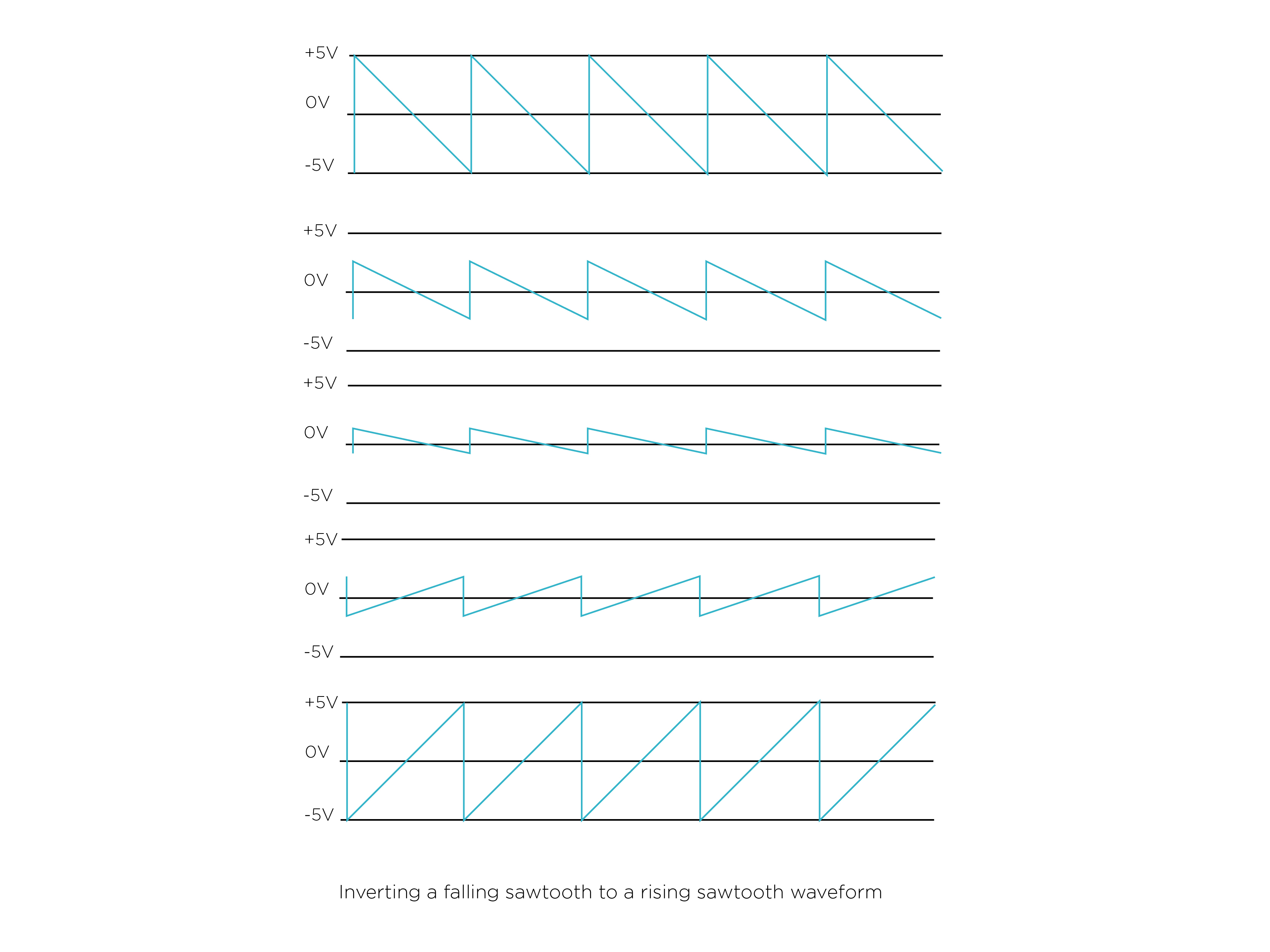
A function that often accompanies an attenuverter on dedicated modules is a voltage offset. Adding an offset to a signal preserves the amplitude while changing the range of the modulation. So if you had an LFO that oscillates between +2.5V and -2.5V, offsetting it by +2.5V would give you a range of 0V to +5V. One useful example of this technique could be sending an LFO through an attenuverter and offset and then to a filter. The offset sets the base cutoff frequency, while the attenuverter sets the strength and polarity of the modulating signal that oscillates around the base cutoff frequency. Modules that have dedicated attenuverters on the CV inputs and panel controls function similarly to dedicated offset/attenuverter modules.
Simple + Useful Voltage Processors

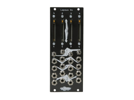 Noise Engineering Lapsus Os Voltage Processor (Black) 10hp$260.00Preorder Reserve your order today!
Out of Stock
We're awaiting our next batch of this item. Pre-order to reserve your place in line and we'll fulfill your order as soon as we receive our shipment ALM Busy Circuits O/A/x2 Dual Offset Attenuverter 4hp$100.00Preorder Reserve your order today!
Out of Stock
We're awaiting our next batch of this item. Pre-order to reserve your place in line and we'll fulfill your order as soon as we receive our shipment
Rectification
Rectification is another form of amplitude processing that alters the polarity of CV signals. Rectification comes in two forms: half-wave and full-wave. In either case, rectification converts bipolar signals into unipolar signals. In other words, a rectifier is used to convert signals with both positive and negative voltage components into signals with only positive polarity. Half-wave rectification simply clips any negative voltages, making that portion of the signal 0V. Full-wave rectification folds any negative voltages up into the positive realm. When full-wave rectifying a periodic waveform such as a triangle wave, you essentially double the frequency by continuously folding the waveform into the positive realm. This is not always the case, particularly with aperiodic waveforms, such as random voltage generators.
The Plum Audio Rect and ADDAC208 offers half-wave and full-wave rectification in both the positive and negative realms, a configuration not found on most rectifiers.
Rectifiers Galore
 Noise Engineering Pura Ruina Distortion 10hpAs low as $260.00Multiple Options Make a selection for stock info
 Plum Audio RECT 1U Wave Rectifier 10hpAs low as $69.00Multiple Options Make a selection for stock info
 ADDAC System ADDAC208 Comparator & Rectifiers 4hp$149.00Out of Stock Sign up for stock updates!
Out of Stock
We aren't currently accepting pre-orders for this item. Sign up for stock notifications and we'll email you as soon as we receive our next shipmentOut of stock
Mixing and Voltage Addition
Another way to take simple modulation sources and add complexity via simple voltage processing is to mix them. Mixing multiple modulation sources creates new, unique modulation, even more complex than its constituent parts. Mixers such as the Roti Pola from Noise Engineering offer four channels of mixing with attenuverters. With nothing patched into the first input, the attenuverter adds or subtracts a static offset. Mixing two out of phase LFOs helps create a new waveform, which may almost seem random based on the phase and frequency relationship between the signals. Or use the method of LA's own Baseck—mix a sequence with a percussive exponential envelope and noise into an oscillator's pitch CV input to create dynamic percussive results.
A matrix mixer adds even more modulation mixing possibilities. A matrix mixer has a set of inputs and outputs, typically arranged into rows and columns. A signal passes from the inputs along the row it occupies. At each intersection of a row and column, a potentiometer sets the signal strength. The matrix mixer mixes each of the columns based on their amplitude. This takes four independent modulation sources and combines them to create four more related, complex modulation sources. Modules such as the 4ms VCAM, or VCA Matrix, combine matrix mixing with amplitude modulation, which we'll cover in the next section.
Some of Our Favorite CV Mixers
 Noise Engineering Roti Pola Attenuverting Mixer (Black) 4hp$160.00Preorder Reserve your order today!
Out of Stock
We're awaiting our next batch of this item. Pre-order to reserve your place in line and we'll fulfill your order as soon as we receive our shipment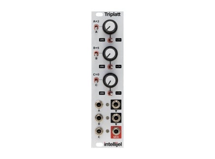 Intellijel Designs Triplatt Mixer + Voltage Utility 6hp$109.00Preorder Reserve your order today!
Out of Stock
We're awaiting our next batch of this item. Pre-order to reserve your place in line and we'll fulfill your order as soon as we receive our shipment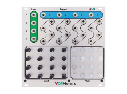 4MS VCA Matrix 26hp$375.00Preorder Reserve your order today!
Out of Stock
We're awaiting our next batch of this item. Pre-order to reserve your place in line and we'll fulfill your order as soon as we receive our shipment
VCAs and Voltage Multiplication
Up until now, we've touched on manual modulation processing, but modulating your modulators opens up new realms of possibilities. VCAs (voltage-controlled amplifiers) are an essential part of modular synthesizers, allowing users to automate amplitude changes with control voltage. Most commonly, VCAs control an audio signal's amplitude, but many VCAs also accept CV signals. This allows you to automate the amplitude of a modulation source in order to vary it dynamically over time. You can think of this process as similar to simple attenuation, and in fact, it's fair to think of a VCA as a voltage-controlled attenuator—one whose attenuation level is automated by another control voltage.
Combining signals with a mixer uses voltage addition, simply adding voltages to get their sum. VCAs, on the other hand, multiply voltages. The most common implementation is the two-quadrant multiplier, usually referred to as a VCA with no qualifier. A four-quadrant multiplier offers bipolar amplitude modulation, sometimes referred to as ring modulation or voltage-controlled polarization. Two quadrant multiplication vs. four-quadrant modulation can be thought of in similar terms as the difference between an attenuator vs. an attenuverter. Some VCA modules also include mixers, combining voltage multiplication with addition.
Modulating and automating the depth of modulation adds new control possibilities to your patches. Use an envelope with a slow attack stage and fast decay to modulate the amplitude of an LFO patched into an oscillator's pitch for slowly evolving and ramping up vibrato that cuts out suddenly. Patch a random voltage generator into a VCA and then use a gate signal to completely turn on or off the random modulation at a synced or unsynced interval. Modulate the amplitude of a sequencer's CV output with another sequencer of a different step length for sequences that change over a period based on the relationship between the two step lengths and amplitude levels. VCAs offer countless ways of manipulating audio and CV—for more tips about creative uses of VCAs, be sure to check our in-depth exploration into VCAs here.
Time Domain Processing: Slew and Lag
We switch now from CV processing in the amplitude domain to CV processing in the time domain. Instead of changing the level of CV signals, time-domain processing introduces variation in the rate of change of CV signals, smoothing them out or introducing a delay between voltage levels.
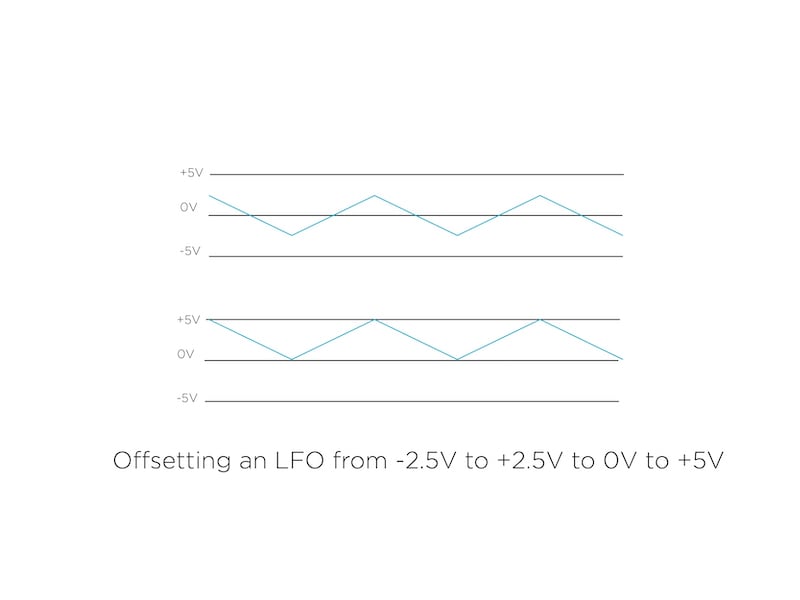
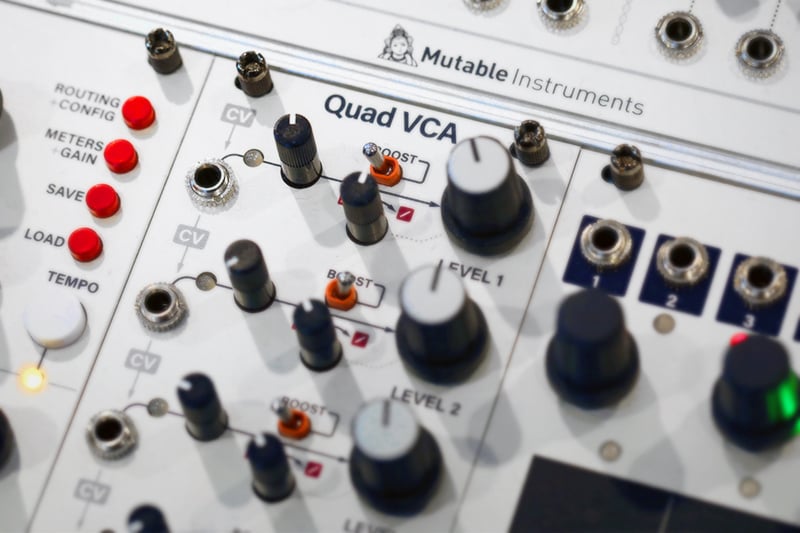
[Above: detail of Make Noise's Maths, a popular Eurorack module composed of two slew limiters and a variety of other CV processing tools.]
A slew limiter limits the maximum rate of change for a voltage over time with a function called integration. The process goes by many names, including slew, glide, portamento, or lag. Slew typically comes in two forms: a single control for slew time or a two-stage control of slew. The single-control slew generator sets the slew amount for any transitions between levels. A two-stage slew generator allows for independent control of the time it takes to travel up or down to a particular voltage level.
With the most common type of one-stage glide, linear constant rate, the larger the interval between voltages, the longer the time it takes to move from one to the next. With linear constant time, the glide time stays constant regardless of the change in voltage. Slew also comes as exponential, starting gradual and speeding up over time, or the inverse, logarithmic, which slows down over time. Often two-stage slew includes the ability to variably change the glide curve, from logarithmic to linear to exponential, sometimes independently between rise and fall.
One way to think of a slew generator is like a low pass filter but for CV, smoothing out a signal's harsh edges at a specified time or frequency range. While similar to a low pass filter, slew generators generally lack resonance and impart different harmonic characteristics to the incoming signal.
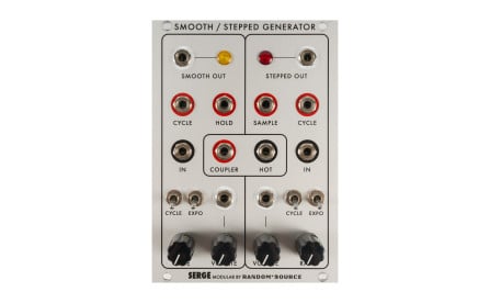
The most common application of slew is adding it to a stepped voltage source such as a sequencer or random voltage generator such as a sample and hold. Adding slew slows down and smooths out the changes between voltage levels, providing a continuously varying voltage based on slew time instead of sudden staircase-like steps. Many instruments, from trombones to violins to the human voice, often don't feature sudden jumps between notes. Adding slew to stepped voltages sometimes adds a slightly more organic quality to them that mirrors many acoustic instruments. Adding slew to a square wave or gate signal turns it into a smoothed sawtooth, triangle, or trapezoidal waveform, depending on the pulse length, curve, and slew time. Often users implement this resulting waveform as an envelope.
Popular Slew Limiter Modules
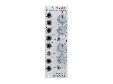 Doepfer A-171-2 Voltage Controlled Slew Processor / Generator 8hpAs low as $149.99Multiple Options Make a selection for stock info
Highlights: a Few Outstanding Eurorack Voltage Processors

Of course, voltage processors come in loads of shapes and sizes—we've included links to several throughout the rest of this article, but also wanted to reserve some space to talk about a few of our favorites. Of course, what you do with a voltage processor can vary widely from patch to patch...so here, we'll talk about a few favorites that offer an uncommon level of flexibility.
The 4MS SISM, or Shifting Inverting Signal Mingler, is a four-channel CV and audio processor that combines offset, attenuversion, and mixing to transform incoming signals. Each of the four channels features bipolar control of Scale (attenuversion) and Shift (offset) and individual outputs. The module then mixes all four channels and sends them to the output section. Mix outputs the sum of all channels, while Mix SW (switch) outputs any channel that does not have a jack currently inserted. + Slice outputs the positive-going signals, while -Slice outputs the negative-going signals. The fourteen LEDs indicate signal strength and polarity, with red indicating positive voltages and blue indicating negative voltages.
 Befaco A*B+C Voltage Processor 6hpNo Longer Available Contact us for a recommendation.Out of stock
The Befaco A*B+C also combines signal addition and four-quadrant multiplication in order to process several CV sources. The module multiplies the A input signal by the B input, and then adds that result to the signal present at the C input. Both the B and C channel features a static voltage offset normalled into their inputs, allowing the module to function with only one signal input signal present. The four-quadrant multiplication offers bipolar control over signal amplitude, plus mixing with a tertiary signal present at the C input. Not only that, but the top section features normalization to the input of the bottom section for mixing the two together. Use the A*B+C as an attenuverter and offset, bipolar VCA with offset, or as a way to combine multiple signals of varying amplitude and polarity to produce a new, related signal of increased complexity compared to the constituent input signals. Also, unlike many attenuverters, A*B+C will amplify signals beyond unity gain—so you can actually use it to increase a signal's amplitude.
The defacto amplitude and time-domain processing powerhouse in Eurorack is the Make Noise Maths. While it is often relegated to the function of dual LFO or dual envelope, digging deeper into the functionality of Maths unlocks new processing possibilities. It covers many of the functions described, including attenuverting, offsetting, mixing, rectification, multiplication, and two-stage slew limiting. Channels 1 and 4 offer two-stage function generators with controls for rise, fall, and response (shape from logarithmic to linear to exponential). Channels 2 and 3 include an attenuverter with a voltage normalled in for offsetting signals. All four channels pass into the mixing section which features a sum (mixed), inv (inverted mixed), and OR, which passes the highest signal present at the mixer. Patching out from any one of the individual signal outputs removes it from the mixing section.
To explore the time domain functions, patch a varying stepped signal from a sequencer or random source to the main signal input on channel 1 or 4. Use the rise and fall parameters to set the speed of the time-domain processing. Dynamically alter the time range with external modulation signals, such as the opposite function generator on Maths, a related secondary signal coming from the module patched into Maths, or a completely unrelated signal. Incorporating channels two and three into the external modulation source gives a new level of amplitude domain processing and finer control over the modulation range. While Maths offers many processing functions on its own, patch programming offers deeper synthesis and processing opportunities. Patch programming is a technique wherein using patch cables within a single module changes the functionality based on the new connections. For example, to patch a full-wave rectifier, mult a signal to both channel 2 and 3, set one attenuverter all the way positive (clockwise), set the other all the way negative (counterclockwise). The full-wave rectified signal is then available at the OR output.
These examples are just a few ways to implement CV processing. Experiment with any one of these techniques, or combine several of them to your tastes. CV processing helps transform your otherwise static modulation sources into new entities with plenty of room for exploration and customization to unlock new modular possibilities.