Frequency modulation is a classic synthesis technique that involves modulating one oscillator's frequency with another, generating complex waveforms from just two (or more) signals. Popularized by John Chowning’s 1970s discovery of FM’s ability to generate rich, natural-sounding timbres through audio-rate modulation, FM (and its frequently conflated counterpart, phase modulation) revolutionized digital sound design at a time when computing power was limited. FM allowed complex, evolving tones to be produced with just a few components. Chowning’s breakthrough—which was licensed by Yamaha for the DX7, the best-selling synthesizer of all time—has had an enduring appeal because of its ability to create both harmonic and inharmonic spectra, capable of producing everything from warped bell tones to glossy basslines. It’s also a technique that occurs very intuitively in a hardware synthesis workflow, where different forms of modulation (and especially audio-rate modulation) are staples.

In Part 1 of this two-part series we explored FM through an intuitive analogy, using the unit circle to visualize a sine wave. Imagining a sine wave as a point tracing the circumference of a unit circle at constant speed, we imagined frequency modulation as the speed of this point constantly changing according to a second signal, creating compressed and stretched waveforms, and producing additional frequencies, known as sidebands. The arrangement and intensity of these sidebands determine the character of the resulting sound. Additionally we explored the history of frequency and phase modulation, from Chowning to modern VSTs, such as Serum 2.

×

[Figure 1: A sine wave (or cosine wave) is the horizontal projection of uniform circular motion—unwrapped along the time axis.]

In Part 2 of this series we’ll continue this intuitive exploration of frequency modulation concepts by examining several specific forms and techniques of FM synthesis.

We’ll start by comparing linear and exponential FM, clearly explaining how each affects pitch stability, tuning, and overall sound quality. Next, we'll explore through-zero frequency modulation (TZFM), a synthesis technique where the modulating signal can reduce the instantaneous frequency of a carrier oscillator below zero. Rather than clamping at zero hertz, as in conventional analog FM, TZFM allows the oscillator to produce “negative frequencies,” which mathematically corresponds to a reversal in the direction of phase accumulation. This ultimately preserves the continuity of the signal and enables a greater range and richness of frequency modulation. TZFM is ideal for creating dynamically rich, harmonically complex textures.

Finally, we'll explore multi-operator FM synthesis. Using classic examples like Yamaha’s DX7 as well as modern hardware synthesizers, we’ll see how combining three or more oscillators, often with their own amplitude envelopes, can create more spectral richness.

As in Part 1, the goal here isn’t to dive deep into the formal mathematics of frequency modulation. Instead, we’ll use analogy as a tool for clarity. The goal is to make these mathematically rich ideas accessible without diluting their complexity.

Linear vs. Exponential Frequency Modulation

Although the terminology is still relatively unfamiliar in the digital VST world, you may have seen hardware oscillators like the Steady State Fate Zero Point Oscillator and Joranalogue Generate 3 which have both exponential and linear FM inputs. What exactly is linear or exponential about FM?

“Linear” and “exponential” are mathematical terms that describe different types of relationships between variables. A linear relationship means that a change in one variable produces a proportional change in another. In contrast, an exponential relationship involves multiplicative change. Instead of rising by equal steps, the values grow (or decay) at an accelerating rate—small at first, but quickly increasing as the input increases.

To illustrate this difference, imagine an oven-temperature dial. On a linear dial, turning the knob 50% of the way would yield a temperature exactly halfway between the minimum and maximum—say, 250°F on a 0–500°F scale. Each additional degree of rotation increases the temperature by the same number of degrees. On an exponential dial, by contrast, each equal increment of rotation increases the temperature by a larger multiple than the last. The first quarter turn might raise the temperature by 50°F, the next by 100°F, then 200°F, and so on. This models exponential growth—slow at first, then dramatically steeper. It’s not the best design for an oven temperature dial, unless we want our oven to get very hot very quickly!

This relates to frequency modulation where the core idea is that one oscillator—typically called the modulator—is used to continuously alter the instantaneous frequency of another oscillator—the carrier. The terms “linear” and “exponential” refer to how the modulator’s voltage (or digital value) affects the carrier’s frequency: in linear FM, changes in the modulating signal result in equal additive changes in frequency, while in exponential FM, those same changes result in multiplicative changes in frequency.

Linear Frequency Modulation in Detail

Let’s look at linear FM first. In linear FM, one oscillator—the modulator—is used to nudge the frequency of another oscillator—the carrier—up and down. Let’s assume the modulator oscillator has a fixed frequency, say 100 Hz, meaning it completes 100 cycles per second. What changes is the modulation depth—how much it affects the carrier. For example, if the depth is set so that it pushes the carrier frequency ±100 Hz, then a 440 Hz carrier gets pulled as low as 340 Hz and as high as 540 Hz by the modulator. Crucially, these shifts are symmetrical and additive. Even as the carrier’s frequency swings from its low boundary to its high boundary, its average pitch remains fixed at 440 Hz.

To visualize linear FM, imagine a point rotating steadily around a unit circle. The carrier’s frequency corresponds to the speed of this rotation—one full spin per cycle of the waveform. Now imagine a modulator oscillator gently tugging on that speed, pushing it faster and slower in a repeating cycle. In linear FM, those pushes and pulls are equal and opposite. This balance ensures that the average rate of rotation averages out to be the same as the carrier's original rate of rotation or frequency, even as the shape of the orbit becomes more intricate. The point (representing the waveform in our analogy) still orbits at the same overall rate. But the path around the circle deforms dynamically, stretching and compressing, which creates sidebands and the perception of a new emergent timbre. The waveform’s shape evolves, but its average and perceived pitch remains constant.

This is very useful when you want to change the timbre of an oscillator without straying too far from a pitch center or harmonic reference point. If you want your music to be in a key, or at least in a scale, linear FM allows you to sculpt harmonically rich sounds without breaking the musical context, and this is one reason that, in the digital domain, linear FM (and similar phase modulation) have been used most commonly.

Let’s say your carrier is tuned to 440 Hz. If the modulating signal increases by a certain amount, it might double the carrier’s frequency to 880 Hz—an octave up. If the modulating signal decreases by that same amount, it might halve the frequency to 220 Hz—an octave down. That seems symmetrical: equal input changes in either direction lead to equal pitch intervals. But if we look at the actual frequency values, doubling from 440 Hz adds 440 Hz, while halving subtracts only 220 Hz. The upward swing introduces a larger frequency change than the downward swing.

This asymmetry leads to a net upward shift in average frequency as the modulation depth increases. Even if the modulator is a perfect sine wave centered around zero, the carrier ends up spending more time being pulled upward than downward. The result is that the perceived pitch drifts higher, even though the modulating signal is balanced.

Exponential Frequency Modulation in Detail

It’s not about the frequency of the modulator; it’s about how the carrier responds to it. In exponential FM, the carrier interprets input changes as ratios—like octaves or semitones—rather than raw frequency shifts. This makes exponential FM well-suited to effects like vibrato, where a small up-and-down movement results in a natural-feeling pitch wobble. But as modulation depth increases, the imbalance becomes more extreme, and the pitch center rises. This makes exponential FM powerful for sound design and interesting textures, but harder to control in harmonic or tonal music.

This brings us to a key historical and technical detail: most analog synthesizers implement exponential FM by default, even if it’s not labeled that way. That’s because hardware synths, especially in the Eurorack and Moog traditions, follow the one volt per octave (V/oct) standard for pitch control. In this system, increasing the control signal by one volt doubles the oscillator’s frequency—an octave jump up. It’s a simple and musically intuitive mapping that mirrors how we perceive pitch. (Remember that frequency doubles with every octave of perceived pitch change in common twelve-tone equal temperament.)

Given this setup, it’s natural to try modulating one oscillator with another by patching the output of one oscillator directly into another oscillator’s V/oct control-voltage input. This kind of frequency modulation—exponential FM—was being explored in analog systems, such as Buchla synthesizers, long before John Chowning’s formalization of FM synthesis in the 1970s. In fact, one reason exponential FM is so widespread in analog gear is that it requires very little circuitry: just apply a varying voltage to the exponential converter, which is already needed to make the oscillator respond musically to a keyboard or sequencer. So modulating that same input with another oscillator is simply the difference between modulating the V/oct input with audio rather than with control voltage.

Challenges in Analog FM

Implementing linear FM in analog hardware is trickier. Linear FM requires a separate input path that doesn’t interpret changes as musical intervals, but instead treats them as raw, additive shifts in frequency. To do this cleanly, the modulating signal must be precisely offset and attenuated, so that it’s centered around zero and doesn’t introduce pitch drift. This often involves a DC-coupled summing stage that injects the modulator signal directly into the core of the oscillator before the exponential converter.

One common approach in analog circuits is to inject the modulation into the integrator or current source that controls the rate of change in a triangle or sawtooth core. The challenge is that any DC offset in the modulating signal will shift the pitch, so careful biasing is critical. Some analog oscillators offer a dedicated “linear FM” input with a built-in attenuverter for this reason. The Joranalogue Generate 3 Eurorack module takes this a step further by including an AC switch on its through-zero linear FM input. When enabled, the AC switch AC-couples the input, filtering out any DC offset or slow modulation components. This prevents unwanted pitch shifts caused by imperfectly centered modulation sources and makes it much easier to achieve stable, deep linear FM tones.

Because exponential FM fits naturally into the most common architecture of analog oscillators, using the same circuitry designed for V/oct pitch control, it became the de facto standard in hardware synthesis. This widespread adoption wasn’t due to any inherent superiority, but simply because exponential FM was much easier to implement in analog oscillators. In contrast, linear FM, while offering greater pitch stability under deep modulation, remained mostly the domain of digital synthesizers and a handful of specialized analog designs until more recently.

Through-Zero Frequency Modulation

Linear FM already fixes the problem of adding modulation while maintaining pitch stability, but it hits a wall. Once modulation pulls the carrier’s frequency down to zero hertz, most analog oscillators stall. There’s simply no negative frequency in a traditional analog oscillator design. Through-zero (sometimes written as “thru-zero”) FM overcomes this by letting the oscillator conceptually pass through zero hertz into “negative frequencies.” But what is a negative frequency?

×

Confusion about through-zero frequency modulation is nearly as old as the concept itself. In Issue #113 of Electronotes, published in May 1980 (a groundbreaking newsletter and DIY engineering journal started in 1972 that served as a hub for analog synthesis experimentation throughout the 1970s and 1980s) long-time editor Bernie Hutchins responded to a reader’s question about the feasibility of negative frequencies. Hutchins, a key figure in the early synth DIY scene and a former Cornell electrical engineering professor, offered one of the first technical clarifications of through-zero FM in print.

In his landmark 1973 paper The Synthesis of Complex Audio Spectra by Means of Frequency Modulation, John Chowning treated negative frequencies as simply a mathematical inevitability of sinusoidal modulation—interpreting them as a reversal of phase direction within a continuously defined waveform. In the digital domain, the distinction between positive and negative frequency is not about direction of movement in a physical oscillator, but about the sign of the rate of phase accumulation. A negative frequency corresponds to a phase rotation in the opposite direction on the unit circle—clockwise instead of counterclockwise. Crucially, this allows the signal to pass “through zero degrees” without discontinuity, preserving the waveform’s shape in mirror image and allowing for symmetrical modulation sidebands no matter where on the unit circle the carrier is centered.

This has real sonic consequences. The result is a richer, more symmetrical frequency spectrum, especially under audio-rate modulation. You retain the full depth of modulation, but the carrier’s pitch center stays stable. The result is a richer, more symmetrical frequency spectrum, especially under audio-rate modulation. Because it preserves pitch stability even at extreme modulation depths, TZFM lets you explore dense harmonic complexity without the tone dissolving into dissonance or chaos. There’s a lot of timbral richness to explore, from crystalline metallophone resonances to throaty vocal textures that remain centered and musically usable.

Slow modulation introduces a distinct character: as the modulator crosses zero, the carrier’s waveform inverts and reassembles, producing a kind of harmonic Doppler effect. Even subtle TZFM can add a breathy shimmer or dynamic instability, acting like an analog chorus or vibrato. When paired with waveshaping or wavefolding, TZFM is capable of everything from percussive clangs to evolving drones and lush harmonic pads.

One of the most powerful artistic uses of TZFM lies in its dynamic potential. Because pitch remains stable, you can modulate the modulation index freely—using envelopes, sequencers, or touch controls to “play” the depth of FM in real time. Modulating the modulator adds motion and tension. There’s also a lot more range available at your fingertips when you get hands on with the modulation. Through-zero inputs can be played with something as simple as a DC offset to become an expressive performance interface.

With the abundance of through-zero FM options available today, it’s easy to forget how recent this explosion of analog capabilities really is. Back in the 1980s, digital modulation was the star. Digital synthesis offered capabilities that analog designers found difficult to replicate. Analog oscillator cores are bound by physical behavior. To achieve through-zero modulation, an analog circuit would need to reverse the direction of its waveform—like making a ramp or triangle wave run backwards in time. That’s easy to model digitally but complex to implement in hardware. In most analog oscillators, once the control voltage pushes the carrier frequency toward zero, the waveform either stalls, flattens out, or becomes unstable. It doesn’t reverse direction. As a result, the modulation symmetry collapses, limiting the depth and fidelity of linear FM.

You also can’t just fake through-zero on an analog oscillator by inverting the output when the carrier signal goes negative. That might flip the waveform, but it doesn’t produce the same phase behavior. What true through-zero FM requires is an oscillator core that literally reverses its phase direction in response to the sign of the control voltage. One way to understand this is by thinking in terms of time. A negative frequency corresponds to reversing the passage of time in the oscillator’s phase evolution. The waveform keeps moving, but in reverse.

12hp

EN129 Thru-Zero Oscillator

$402.00

In stock

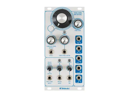
One of the earliest well-known working designs for an analog through-zero oscillator came from Bernie Hutchins in the 1981 issue. Inspired by an earlier concept from engineer Douglas Kraul, Hutchins set out to solve the problem most analog oscillators couldn’t touch: how to make a waveform truly reverse direction when the modulation signal crosses zero. Not just flip upside down, but actually run backward in time—producing what we call “negative frequency” behavior. The heart of Hutchins’ circuit is a simple triangle-wave oscillator. Like many analog designs, it charges a capacitor to make a rising slope, then discharges it to fall again. But here’s the key: the direction of that ramp isn’t fixed. It depends on the polarity of the input voltage. When the control signal goes from positive to negative, a clever bit of circuitry detects the crossing point and flips a digital switch (a flip-flop), which reverses the ramp direction. So instead of stopping or glitching at zero, the oscillator’s trajectory smoothly reverses course. While the Hutchins design wasn’t made commercially available at the time, in recent years, it’s been reimagined in the Dannysound/Tobinski EN129 Eurorack oscillator, which brings the full through-zero experience into the hands of today’s modular musicians.

Through-Zero FM Through the Ages

Through the late 1970s, articles by Hutchins, Jan Hall, and others further refined TZFM theory, but the concept remained largely underground. While Yamaha’s DX7—released in 1983—became the first mass-market FM synthesizer, as we saw in Part 1, it achieved its sounds via digital phase modulation, not analog frequency modulation. Crucially, its digital implementation naturally allowed negative phase increments—effectively a kind of through-zero modulation—though the term was never applied to it at the time. Throughout the 1980s and 1990s, digital FM (and phase distortion) dominated the industry, while analog manufacturers like Moog and Roland largely ignored through-zero techniques.

Still, the DIY community kept the flame alive. In the 1990s, builders on forums and listservs continued to experiment with through-zero designs, including constructing Hall’s circuits from old Electronotes issues. In 2003, Henry Wamsley published a TZFM sine-core oscillator in EDN Magazine, marking one of the first post-Electronotes public designs. Then in 2005, the analog landscape changed dramatically when Cynthia Webster and Mark Barton released the Cyndustries Zeroscillator, one of the first commercially available analog through-zero FM oscillator. Told that TZFM “could and would only exist in the digital domain,” Barton was driven to prove otherwise, ultimately producing four complete redesigns before a working circuit emerged. The key was the AD734 precision analog multiplier from Analog Devices—a then-$17 chip Barton initially avoided due to cost, but which proved essential. The final module, built from five circuit boards, was released in eight formats—5U, Modcan, MOTM, Eurorack, Frac Rack, Blacet, Buchla, and Wiard—making it arguably the most format-flexible module ever produced. Despite retailing between $750 and $1,200, the Zeroscillator quickly sold out, receiving rave reviews and finding its way into the studios of composers like Hans Zimmer and Junkie XL.

The Zeroscillator’s success sparked a wave of innovation. Legendary synth designer Ian Fritz followed with the Teezer VCO, a stable and accessible DIY design. Other hobbyists such as Jürgen Haible, René Schmitz, Don Tillman, shared their own schematics online. DIYers suddenly had a menu of through-zero choices.

The 2010s brought through-zero FM into the mainstream. The release of Intellijel’s Rubicon in 2012–13 marked a turning point for Eurorack users. It paired high-performance analog through-zero FM with stability and a host of waveshaping options. Meanwhile, Doepfer introduced the A-110-4 in 2014, a no-frills, quadrature TZFM oscillator. More manufacturers followed suit: WMD, Endorphin.es, and Joranalogue released their own takes. Joranalogue’s Generate 3 (2018) showcased fully analog through-zero FM and phase modulation with modern precision.

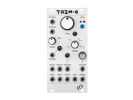
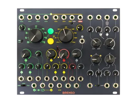
By the late 2010s and into the 2020s, through-zero FM was no longer esoteric. Instruō’s Neóni, for instance, introduced a refined analog TZFM in a compact Eurorack package with built-in wavefolding. In 2022 two very compact through-zero oscillators were released: Befaco released the PONY VCO—an analog, through-zero oscillator packed into just 4hp, and that same year Nonlinearcircuits introduced the FM OP, another 4hp through-zero Eurorack module built around the SSI2130 chip (a hybrid analog-digital design). Likewise, TAZM-O is ALM's take on an SSI2130-fueled thru-zero oscillator, offering continuously variable waveshape and a clean, spacious layout. The Frap Tools Brenso Eurorack oscillator and Magnolia keyboard synthesizer also offer their own takes on the through-zero technique.

Even software platforms started to emulate the analog trend: Cherry Audio released a digital clone of the Zeroscillator in 2023. For a technique that took so much inspiration from the digital domain in the 1970s, it seemed like precision analog FM had oddly come full circle.

As time has worn on, through-zero analog FM has fully transitioned from obscure theory to a respected and increasingly common feature in even very small analog synthesizers. But one of the final frontiers in this evolutionary arc is the notion of “exponential” through-zero frequency modulation.

Thru-Zero-Capable Oscillators

12hp

TAZM-O Analog Through-Zero Oscillator

$420.00

In stock

4hp

Pony VCO 3U Thru-Zero Oscillator

$265.00

In stock

30hp

Brenso Complex Oscillator

$765.00

In stock

Exponential Through-Zero FM: Mathematically Impossible, and Yet…

At first glance, the idea of exponential through-zero FM seems contradictory, and in fact, mathematically, it’s impossible. Exponential FM scales frequency logarithmically with voltage. As voltage decreases, frequency halves again and again, asymptotically approaching zero but never actually reaching or crossing it. In other words, the mathematical structure of exponential FM prevents negative frequency values from ever occurring; there's no meaningful way, in a purely exponential domain, to represent a reversal of direction across zero hertz. From this standpoint, true “exponential through-zero” should be impossible.

And yet, Andrew Morelli, the designer behind the Steady State Fate (SSF) Eurorack brand, managed to do something that flirts with the impossible. Instead of trying to force an exponential core to reverse its frequency, SSF reimagined what it means for an oscillator to move “through zero” in an exponential FM context. The Zero Point Oscillator is a fully analog, discrete triangle-core oscillator with both linear and exponential FM inputs. When through-zero mode is engaged, the incoming modulation signal—whether exponential or linear—is split into two paths. One path runs through a full-wave rectifier before it reaches the frequency-determining part of the oscillator core. This means that negative modulation voltages are flipped to positive, and the core never actually sees a frequency below zero. The other path, however, does something subtler and far more important: it feeds the unaltered modulator into a tuned amplitude modulation circuit—what SSF calls the Zero Point amplifier—that inverts the output waveform whenever the modulator voltage is negative. That inversion mimics what a true negative frequency would do, flipping the oscillator’s phase without requiring the actual integrator inside the oscillator to reverse direction.

The result is something uncanny: even though the core never goes negative, the output behaves as if it did. When the modulation crosses zero, the output flips phase. Over a full modulation cycle, the upward and downward sweeps are symmetrical. The rich sidebands characteristic of through-zero FM are there, and most critically, the oscillator stays in tune—no matter how deep the modulation. In a conventional analog oscillator, deep exponential FM causes the fundamental pitch to drift—because increasing and decreasing voltages push the frequency logarithmically, but not equally. As we’ve seen, positive modulation raises pitch more than negative modulation lowers it. But in the ZPO, the full-wave rectifier removes this asymmetry, and the polarity inversion ensures the sonic outcome remains balanced. It’s not mathematically exponential FM through zero, but perceptually, it achieves a similar result.

At the center of this design is the Zero Point control, which sets the symmetry of the polarity flipping. When set to zero volts—at noon on the knob—the positive and negative swings of the modulator are treated evenly, creating fully balanced through-zero behavior. Tilt it one way or another, and you skew that symmetry, emphasizing either the original waveform or its inverted counterpart, and changing the harmonic structure of the sound. Because the polarity inversion is handled by a VCA-style circuit under voltage control, the depth and symmetry of the through-zero effect can be dynamically modulated as well—allowing envelopes or secondary LFOs to shape not just the FM index but the nature of the TZFM response.

N-OP FM: Modulate More Better Faster

The term n-operator FM (or N-OP FM) might sound arcanine, but you've encountered its simplest form already: 2-operator FM, which is the FM model we’ve described in depth throughout this two-part series. An “operator” refers to the voices involved in FM, such as a carrier or modulator. But in FM synthesis, an “operator” isn’t usually just an oscillator. It’s often a combination of an oscillator, its own envelope generator, and a voltage-controlled amplifier (VCA). In 2-OP FM, one oscillator (the modulator) affects the frequency of another (the carrier). Add a third operator, and things get more interesting. 3-OP FM opens the door to multiple routing possibilities: voice A could modulate voice B, which in turn modulates voice C; or both A and B might modulate voice C in parallel, for example.

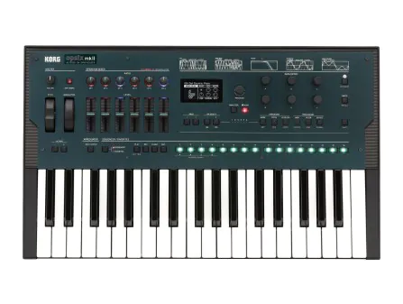
Beyond 3-OP FM, things scale rapidly. 4-OP, 6-OP (as found in Yamaha's DX series and the Korg Opsix), and even 8-OP FM systems, used in Native Instruments FM8, allow for deeply complex operator networks, often with feedback paths. There are even FM matrices built in the SuperCollider programming language where arbitrary numbers of oscillators can modulate and feed back their modulation on themselves and each other in complex-to-model ways.

While high-order n-operator FM is relatively rare in analog synthesis, digital synthesis has employed this form of FM modulation from the very beginning. Yamaha DX7, one of the best-selling synths in history (technically a phase modulation synth, as we saw in Part 1), featured six sine-wave operators per voice that could be arranged into 32 “algorithms,” preset routings that defined which operators modulated which and whether feedback was used. Each algorithm, which was printed as a pictogram on the DX7, is in effect a map of signal flow: which operators act as carriers, which as modulators, which are arranged in series, in parallel, or provided with feedback. Some configurations were relatively simple. Others were more layered or branching, with multiple modulators influencing a single carrier, or long chains where one operator modulated the next in sequence. Each operator had its own envelope generator, allowing independent control of amplitude over time. That meant a modulator could rise quickly and decay, while its carrier held a long sustain.

×

[Figure 2: Front panel of the Yamaha DX7II-D showcasing its 6-operator FM synthesis structures. Credit: Photo by deepsonic, licensed under CC BY 2.0.]

In response to the complexity inherent in programming this kind of synthesizer, in 1986 John Chowning and Yamaha consultant David Bristow published FM Theory and Applications, a book that drew on, not only their expertise designing modulation presets, but also exclusive technical insights into the DX7’s inner workings, made possible by Yamaha’s direct support. The book compares several different types of signal flow which are possible with n-operator FM:

Cascade (Series) Configuration: Operators are arranged in a chain where each modulates the next, and only the final operator (the carrier) produces audible output. Each added modulator stage exponentially increases spectral complexity by generating dense sidebands, often yielding sharp, metallic, or bell-like timbres with rich inharmonic content.

Parallel Configuration: When multiple modulators simultaneously feed a single carrier (parallel modulators), their output waveforms combine arithmetically before affecting the carrier. This means the resulting spectrum is a blend of all harmonic contents from each modulator. Individual carriers may each be modulated by their own stack of modulators or left unmodulated. Conversely, when a single modulator feeds multiple carriers in parallel, it modulates each carrier independently. Each carrier produces its own waveform, possibly with distinct frequency ratios or envelopes, creating a layered texture where individual carriers contribute unique timbres. This approach resembles additive synthesis but is uniquely dynamic due to FM’s evolving sidebands, producing a rich interplay of independent harmonic structures.

Feedback Configuration: Some algorithms route an operator’s output back into itself or into another modulator’s input. This feedback loop rapidly intensifies spectral complexity, turning simple sine waves into harmonically rich “bristling” tones or even noisy textures at high feedback levels. While feedback enables aggressive and percussive sounds, it demands careful control to avoid instability or distortion.

The interplay between series, parallel, and feedback configurations becomes especially potent when considered in light of the operator envelopes. Each operator’s amplitude can evolve independently over time, meaning that the depth, spectral focus, and even the existence of certain frequency components can shift as the note progresses.

Reflecting on his work designing 6-operator FM algorithms for Yamaha, Bristow noted in an interview with Electronics & Music Maker magazine in 1983 that the complexity of these algorithms requires both experimentation and intuition. Bristow encouraged users to listen systematically, turning operators on and off to isolate their contributions, then gradually building complexity:

[You start] by listening to an FM pair and see what they do. A pair refers to the vertical in-line Operators. Then you start listening to three Operators. More than this would be too much to take in at the first attempt because the ratios become too complicated. You always start at the bottom of the algorithm diagram because that's where the sound originates from—the carriers. It's impossible for the mind to retain all the different values, but you get a feel for how things sound.

Although 3-operator FM is theoretically simple to achieve in hardware synthesizers by simple modulating a modulation oscillator (or voice) with another oscillator, high-order n-operator FM is difficult to manage in hardware synthesizers for the same reasons that make polyphonic music difficult to achieve in hardware systems: the complexity of the system, involving potentially an oscillator, envelope, and VCA for every operator (not to mention modulation for the same) rapidly multiplies with every additional operator added to the mix.

An additional challenge is that, to achieve certain harmonic or inharmonic timbres, the modulator (or modulators) must remain in a precise interval ratio to the carrier frequency. These simple ratios are what produce harmonic sidebands, resulting in musically consonant tones. But even slight detuning—whether due to oscillator drift, temperature fluctuations, or imperfect tracking—can shift the relationship away from these ideal ratios, causing the resulting spectrum to become increasingly dissonant or noisy. As more operators are added in n-operator FM structures, the difficulty compounds: each modulator must remain in tune not only with the carrier, but with other modulators as well.

A number of digital hardware synthesizers have taken on the challenge of 3-operator FM synthesis. Industrial Music Electronics was among the first, with their Hertz Donut series of digital FM oscillators inspired by the Buchla 259e Complex Oscillator. The newest version of the Hertz Donut (now in its MkIII incarnation) expands on the Buchla concept by adding a third internal modulation operator and an external FM bus—which can run in series or in parallel—significantly enhancing the depth and variety of achievable timbres with phase distortion, and fractal "umbrage," and bringing the concept to the compact Eurorack format.

More recently, the Schlappi Engineering Three Body has emerged as a modern incarnation of 3-operator FM synthesis for Eurorack users. The Three Body takes the foundational principles of multi-operator FM and pushes them forward with advanced features such as complex algorithm selection, flexible feedback paths, and expanded modulation possibilities including both frequency and phase modulation with through-zero capabilities. Its three oscillators can operate independently or in tightly integrated ratio tracking modes, allowing classic Chowning-style harmonic relationships or free-running complex textures. The module’s high internal sample rate (12.5 MHz) and 16-bit quality with 96kHz sample rate ensures pristine, aliasing-minimized sound. Additional unique features include multiple simultaneous waveform outputs per oscillator (sine, cosine, triangle, saw, and square) and configurable phase modulation directions for stereo effects.

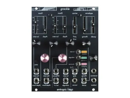
A relatively recent addition to the 3-operator Eurorack landscape, Entropic Loop’s Grackle offers a fresh take on phase modulation synthesis with three oscillators featuring additive, multiplicative, and cascade routing algorithms. Its unique interval system uses just-intonation-inspired fractional ratios for rich harmonic complexity. A versatile envelope generator with triggered, cycling, and asymmetric slew modes provides expressive dynamic shaping. With CV-normalled modulation depths and thru-zero frequency modulation support, Grackle (like the Schlappi Three Body) delivers digital precision with an immediate-feeling, screen-free interface that almost feels analog.

Modern Multi-Operator FM Modules

20hp

Grackle 3-Operator FM Voice

$600.00

In stock

30hp

Three Body Triple FPGA Oscillator

$595.00

In stock

17hp

Hertz Donut MKIII Digital FM Oscillator

$525.00

In stock

Conclusion

As much as analog synthesis has shaped the aesthetics and workflows of electronic music—through the postwar experimentalism of Cologne and Paris, the tactile and voltage-controlled systems of Moog and Buchla, and the patch-programmable philosophy Serge—it’s striking how many of analog FM’s recent advances have their roots in digital synthesis.

In Part 1, we explored FM’s conceptual foundations, the overlap between frequency and phase modulation, and how John Chowning’s discoveries gave rise to the Yamaha DX7 and other digital instruments. In Part 2, we followed those digitally-driven ideas back into hardware, tracing how linear FM, through-zero FM, phase modulation, and even n-operator FM architectures, originally more feasible in software, have found their way into modern analog designs.

It’s easy to take these features for granted today, but for much of electronic music’s history, they were either impractical or unexplored. Many of the breakthroughs that brought these digital techniques into the analog world emerged quietly on internet forums, in DIY hobbyist newsletters, and in one-off designs that never saw wide circulation. It’s remarkable that a constellation of synthesis techniques which gained traction in the 1980s partly because of their efficient use of limited digital processing power not only remain relevant today, but have dramatically expanded in technical and artistic potential—especially in the analog domain—even as digital synthesis has grown to include so many new approaches, such as wavetables and physical modeling.

More FM Synthesizers to Check Out

First Love Multitimbral FM Synthesizer

$699.00

In stock

4% offSTAFF PICK

Digitone II 16-Track Polyphonic Digital Synthesizer

Special Price $1,099.00 Regular Price $1,149.00

In stock

Opsix MkII FM Keyboard Synthesizer

$599.99

In stock